How to convert a matrix to a table in Google Sheets
June 19, 2021Motivation
I came across an interesting problem while performing my data engineering duties at work.
I had to import a spreadsheet's content into a relational database. It may sound like a trivial task, but there was a catch: the data was defined in a matrix format.
It looked something like this:

It's a matrix that defines the monthly budget of each department for the first half of 2021.
To import this data into an RDBMS, we need to convert it to a table first.
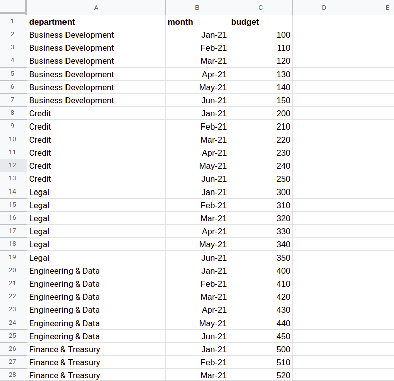
The transformation should be dynamic, so when the matrix is updated, the changes are automatically reflected in the table.
I haven't found any articles on the subject, so I think my solution is worth sharing.
Helper tables
To make our lives easier, let's define two helper tables - one for the matrix rows and one for the matrix columns.
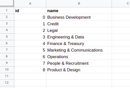
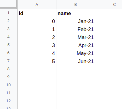
Let's make them truly dynamic, so whenever a new row or column is added to the matrix, it automatically appears in the helper table.
Counting the matrix rows/columns
First, we need a way to count the number of rows/columns in the matrix.
Luckily for us, the COUNTA function will cover 100% of our counting needs.
It's a function that counts all non-empty cells inside a given range:
-
counta(matrix!$A:$A)- count the number of rows (i.e. non-empty cells in column A) -
counta(matrix!$1:$1)- count the number of columns (i.e. non-empty cells in row 1)
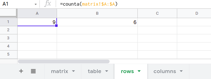
In its current state, the matrix has 9 rows and 6 columns.
Copying the matrix rows
To copy the matrix rows, we can use the ARRAYFORMULA function.
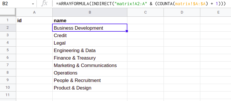
ARRAYFORMULA(INDIRECT("matrix!A2:A" & (COUNTA(matrix!$A:$A) + 1)))This formula:
-
Builds the string
"matrix!A2:A10". This string represents the cell range of the matrix rows. -
If a new row is added to the matrix, the range is automatically increased by one row (because of the
COUNTAfunction). - Then, it converts the cell range string to an actual cell range reference with the INDIRECT function.
- Finally, it copies the cell range reference to the current position with the ARRAYFORMULA function.
Generating ID numbers
To generate ID numbers, we can use ARRAYFORMULA combined with the ROW function.
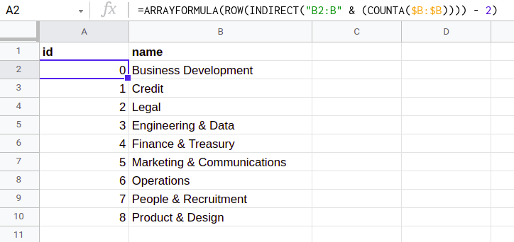
ARRAYFORMULA(ROW(INDIRECT("B2:B" & (COUNTA($B:$B)))) - 2)The idea is similar to copying cells.
-
First, it builds the cell range string
"B2:B10". If a row is added/deleted, this range is automatically adjusted. - Then, it converts the string to a cell range reference with INDIRECT.
- Next, it takes the row number of each cell (with ROW) and subtracts two from all of them, so the resulting sequence is zero-based. We'll see why this is important later.
- Finally, it copies the sequence to the given position with ARRAYFORMULA.
Calculating the last matrix column
To calculate the last matrix column, we can use the ADDRESS function.

address(1, counta(matrix!$1:$1) + 1, 4)The ADDRESS function takes a row and a column number, and returns a cell reference string.
So, in the formula above:
-
1is the row number. -
counta(matrix!$1:$1) + 1is the column number. It will evaluate to7in this example. Column 7 is G. -
4is the flag for returning the address in the format"G1".
Copying the matrix columns
Copying the matrix columns is pretty similar to copying the rows.

transpose(arrayformula(to_text(indirect("matrix!B1:" & address(1, counta(matrix!$1:$1) + 1, 4)))))That's quite a mouthful! Here's what it does:
-
First, it builds the
"matrix!B1:G1"cell range string with the help of the ADDRESS function. -
If a new column is added, the range is automatically adjusted.
For example, if we added the column
Jul-21, the cell range string would be"matrix!B1:H1" - Then, it transforms the cell range string to a cell range reference with INDIRECT, and copies the values to the position with ARRAYFORMULA (as discussed above).
- To make sure Google Sheets handles the values as texts (not as dates), all values are converted to text with the TO_TEXT function.
- Note that ARRAYFORMULA will output the cell range horizontally. To change it to vertical, we need to use the TRANSPOSE function.
Flattening the matrix values
Now that both helper tables are ready, we can start adding columns to the main table.
To make things easier, let's use the FLATTEN function.
The FLATTEN function takes a range of values and flattens them into a single column.
For example:
| 0 | 1 | 2 | 3 |
| 4 | 5 | 6 | 7 |
| 8 | 9 | 10 | 11 |
| 0 |
| 1 |
| ... |
| 11 |
We can use it to extract the matrix values into the main table:
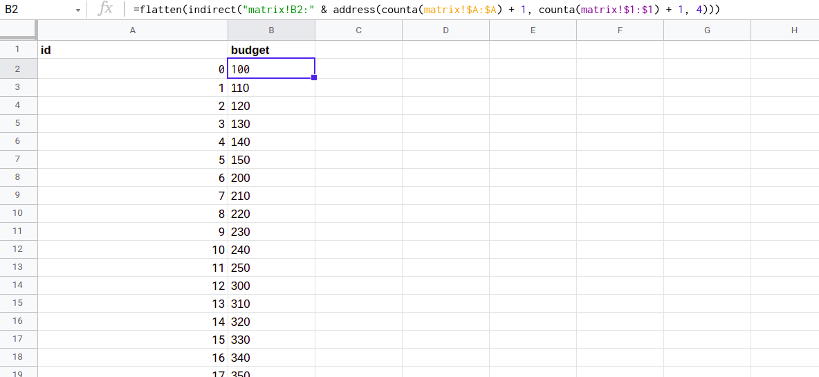
flatten(indirect("matrix!B2:" & address(counta(matrix!$A:$A) + 1, counta(matrix!$1:$1) + 1, 4)))Conceptually, this formula is pretty similar to the previous ones:
-
First, it builds the
"matrix!B2:G10"cell range string with the help of the ADDRESS function. This range includes all matrix values (but not the row/column names). If someone adds a new column or row to the matrix, it is automatically adjusted. - Then, the cell range string is transformed to a cell range reference with INDIRECT.
- Finally, FLATTEN flattens the matrix values into a column and outputs them (similarly to ARRAYFORMULA).
Calculating the row IDs
To calculate which matrix row a given item belongs to, divide the ID with the width of the matrix and discard the remainder (keep the integer part only).
For example:
| 0 | 1 | 2 | 3 | → | 0 |
| 4 | 5 | 6 | 7 | → | 1 |
| 8 | 9 | 10 | 11 | → | 2 |
That is,
- 0, 1, 2 and 3 divided by 4 is 0
- 4, 5, 6 and 7 divided by 4 is 1
- 8, 9, 10 and 11 divided by 4 is 2
The QUOTIENT function is the natural choice for this calculation.
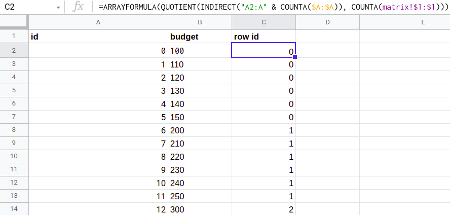
ARRAYFORMULA(QUOTIENT(INDIRECT("A2:A" & COUNTA($A:$A)), COUNTA(matrix!$1:$1)))The formula is pretty straightforward:
-
First, it builds the
"A2:A55"cell range string (referring to the id column) and creates a cell range reference with the INDIRECT function. - Then, the values are transformed with the QUOTIENT function (according to the rules above).
- Finally, the values are copied to the given cell with ARRAYFORMULA.
Calculating the column IDs
To calculate which matrix column a given item belongs to, divide the ID with the width of the matrix and discard the integer part (keep the remainder only).
For example:
| 0 | 1 | 2 | 3 |
| 4 | 5 | 6 | 7 |
| 8 | 9 | 10 | 11 |
| ↓ | ↓ | ↓ | ↓ |
| 0 | 1 | 2 | 3 |
That is,
- 0, 4 and 8 modulo 4 is 0
- 1, 5 and 9 modulo 4 is 1
- 2, 6 and 10 modulo 4 is 2
- 3, 7 and 11 modulo 4 is 3
For this calculation, the appropriate function is MOD.
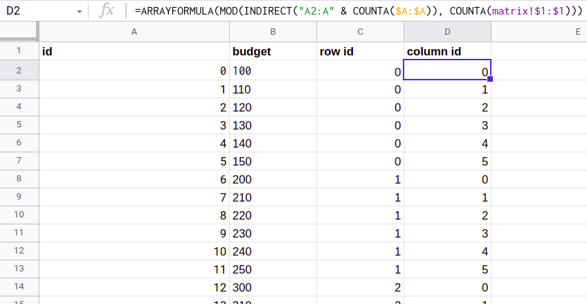
ARRAYFORMULA(MOD(INDIRECT("A2:A" & COUNTA($A:$A)), COUNTA(matrix!$1:$1)))Looking up the rows/columns by their IDs
We're almost done!
We already have the row and column IDs. All that's left to do is to look up the actual values from the helper tables... and when it comes to looking up things, the best in the business is: VLOOKUP.
To put it simply, it's a function for performing a linear search in a table. For example:
VLOOKUP(0, rows!A2:B10, 2) --> "Business Development"Translates to: "find the row name where the id is 0".
The function takes 3 parameters:
0- the id to search forrows!A2:B10- the table to search in2- the column to return
And it can also be combined with ARRAYFORMULA:
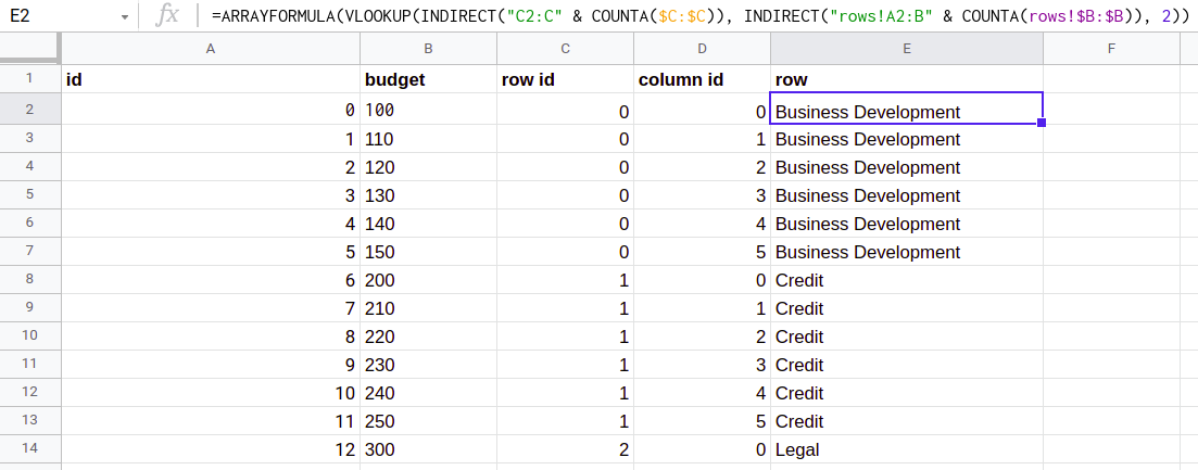
ARRAYFORMULA(VLOOKUP(INDIRECT("C2:C" & COUNTA($C:$C)), INDIRECT("rows!A2:B" & COUNTA(rows!$B:$B)), 2))It looks a bit complicated, but there's actually nothing new here:
-
First, it builds the
"C2:C55"and"rows!A2:B10"cell range references. The first one refers to the row id column, the second one refers to the rows helper table. - We pass 3 arguments to VLOOKUP - the ids to search for, the table to search in and the column to return.
- Finally, VLOOKUP finds the row name for each id and the results are displayed with ARRAYFORMULA.
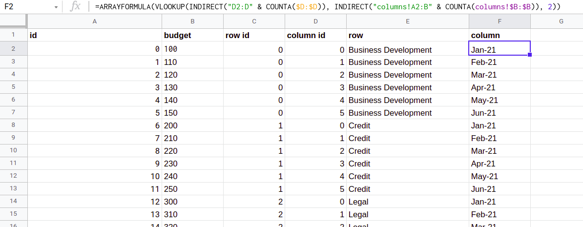
ARRAYFORMULA(VLOOKUP(INDIRECT("D2:D" & COUNTA($D:$D)), INDIRECT("columns!A2:B" & COUNTA(columns!$B:$B)), 2))Conclusion
That's it!
We transformed a matrix into a table using nothing but Google Sheets formulas. Not as easy as it looks!
I hope this post was helpful.